Getting started with Gradient Boosting Machines - using XGBoost and LightGBM parameters

Psst.. A Confession: I have, in the past, used and tuned models without really knowing what they do. I tried to do the same with Gradient Boosting Machines — LightGBM and XGBoost — and it was.. frustrating!

This technique (or rather laziness), works fine for simpler models like linear regression, decision trees, etc. They have only a few hyperparameters — learning_rate, no_of_iterations,alpha, lambda — and its easy to know what they mean.

But GBMs are a different world:

1. They have a huge number of hyperparameters — ones that can make or break your model.
2. And to top it off, unlike Random Forest, their default settings are often not the optimal one!

So, if you want to use GBMs for modelling your data, I believe that, you have to get atleast a high-level understanding of what happens on the inside. You can’t get away by using it as a complete black-box.

And that is what I want to help you with in this article!

What I will do is I sew a very simple explanation of Gradient Boosting Machines around the parameters of 2 of its most popular implementations — LightGBM and XGBoost. This way you will be able to tell what’s happening in the algorithm and what parameters you should tweak to make it better. This practical explanation, I believe, will allow you to go directly to implementing them in your own analysis!

As you might have guessed already, I am not going to dive into the math in this article. But if you are interested, I will post some good links that you could follow if you want to make the jump.

Let’s get to it then..

In the article, “A Kaggle Master Explains Gradient Boosting”, the author quotes his fellow Kaggler, Mike Kim saying —

My only goal is to gradient boost over myself of yesterday. And to repeat this everyday with an unconquerable spirit.

You know how with each passing day we aim to improve ourselves by focusing on the mistakes of yesterday. Well, you know what? — GBMs do that too!

Let’s find out how, using 3-easy-pieces —

1. “An Ensemble of Predictors”

GBMs do it by creating an ensemble of predictors. An army of predictors. Each one of those predictors is sequentially built by focusing on the mistakes of the predictor that came before it.

You: Wait, what “predictors” are you talking about? Isn’t GBM a predictor itself??

Me: Yes it is. This is the first thing that you need to know about Gradient Boosting Machine — It is a predictor built out of many smaller predictors. An ensemble of simpler predictors. These predictors can be any regressor or classifier prediction models. Each GBM implementation, be it LightGBM or XGBoost, allows us to choose one such simple predictor. Oh hey! That brings us to our first parameter —

The sklearn API for LightGBM provides a parameter-

• boosting_type (LightGBM), booster (XGBoost): to select this predictor algorithm. Both of them provide you the option to choose from — gbdt, dart, goss, rf (LightGBM) or gbtree, gblinear or dart (XGBoost).

But remember, a decision tree, almost always, outperforms the other options by a fairly large margin. The good thing is that it is the default setting for this parameter; so you don’t have to worry about it!

2. “Improve upon the predictions made the previous predictors”

Now, we come to how these predictors are built.

Me: Yep, you guessed it right — this is the piece where we see how GBMs improve themselves by “focusing on the mistakes of yesterday”!

So, a GBM basically creates a lot of individual predictors and each of them tries to predict the true label. Then, it gives its final prediction by averaging all those individual predictions.

But we aren’t talking about our normal 3rd-grade average over here; we mean a weighted average. GBM assigns a weight to each of the predictors which determines how much it contributes to the final result — higher the weight, greater its contribution.

You: And why does it do that?

Me: Because not all predictors are created equal..

Each predictor in the ensemble is built sequentially, one after the other — with each one focusing more on the mistakes of its predecessors.

Each time a new predictor is trained, the algorithm assigns higher weights (from a new set of weights) to the training instances which the previous predictor got wrong. So, this new predictor, now, has more incentive to solve the more difficult predictions.

You: But hey, “averaging the predictions made by lots of predictors”.. isn’t that Random Forest?

Me: Ahha.. nice catch! “Averaging the predictions made by lots of predictors” is in fact what an ensemble technique is. And random forests and gradient boosting machines are 2 types of ensemble techniques.

But unlike GBMs, the predictors built in Random Forest are independent of each other. They aren’t built sequentially but rather parallely. So, there are no weights for the predictors in Random Forest. They are all created equal.

You should check out the concept of bagging and boosting. Random Forest is a bagging algorithm while Gradient Boosting Trees is a boosting algorithm.

Simple right?

How does the model decide the number of predictors to put in?
 — Through a hyperparameter ofcourse:

• n_estimators : We pass the number of predictors that we want the GBM to build inside the n_estimators parameter. The default number is 100.

You: But I have another question. Repetitively building new models to focus on the mislabelled examples — isn’t that a recipe for overfitting?

Me: Oh that is just ENLIGHTENED! If you were thinking about this.. you got it!

It is, in fact, one of the main concerns with using Gradient Boosting Machines. But the modern implementations like LightGBM and XGBoost are pretty good at handling that by creating weak predictors.

3. “Weak Predictors”

A weak predictor is a simple prediction model that just performs better than random guessing. Now, we want the individual predictors inside GBMs to be weak, so that the overall GBM model can be strong.

You: Well, this seems backwards!

Me: Well, it might sound backwards but this is how GBM creates a strong model. It helps it to prevent overfitting. Read on to know how..

Since every predictor is going to focus on the observations that the one preceding it got wrong, when we use a weak predictor, these mislabelled observations tend to have some learnable information which the next predictor can learn.

Whereas, if the predictor were already strong, it would be likely that the mislabelled observations are just noise or nuances of that sample data. In such a case, the model will simply be overfitting to the training data.

Also note that if the predictors are just too weak, it might not even be possible to build a strong ensemble out of them.

So, ‘creating a weak predictor’.. this seems like a good area to hyperparameterise, right?
 — “Let’s leave it to the developers to figure out the real problem!” 😛

These are the parameters that we need to tune to make the right predictors (as discussed before, these simple predictors are decision trees):

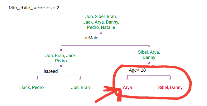
• max_depth (both XGBoost and LightGBM): This provides the maximum depth that each decision tree is allowed to have. A smaller value signifies a weaker predictor.
• min_split_gain (LightGBM), gamma (XGBoost): Minimum loss reduction required to make a further partition on a leaf node of the tree. A lower value will result in deeper trees.
• num_leaves (LightGBM): Maximum tree leaves for base learners. A higher value results in deeper trees.
• min_child_samples (LightGBM): Minimum number of data points needed in a child (leaf) node. According to the LightGBM docs, this is a very important parameter to prevent overfitting.

Note: These are the parameters that you can tune to control overfitting.

Note 2: Weak predictors vs. strong predictors — this is another point of difference between GBMs and Random Forests. The trees in Random Forest are all strong by themselves as they are built independently of each other.

That is it. Now you have a nice overview of the whole story of how a GBM works!

But before I leave you, I would like you to know about a few more parameters. These parameters don’t quite fit into the story I just sewed above but they are used to squeeze out some efficiencies in performance.

I will also talk about how to tune this multitude of hyperparameters. And finally, I will point you some links to dive deeper into the math and the theory behind GBMs.

[Extra]. Subsampling

Even after tuning all the above parameters correctly, it might just happen that some trees in the ensemble are highly correlated.

You: Please explain what you mean by “highly correlated trees”.

Me: Sure. I mean decision trees that are similar in structure because of similar splits based on same features. When you have such trees in the ensemble, it would mean that the ensemble as a whole is going to store less amount of information than what it could have stored if the trees were different. So, we want our trees to be as little correlated as possible.

To combat this problem, we subsample the data rows and columns before each iteration and train the tree on this subsample. Meaning that different trees are going to be trained on different subsamples of the entire dataset.
Different Data -> Different Trees

These are the relevant parameters to look out for:

• subsample (both XGBoost and LightGBM): This specifies the fraction of rows to consider at each subsampling stage. By default it is set to 1, which means no subsampling.
• colsample_bytree (both XGBoost and LightGBM): This specifies the fraction of columns to consider at each subsampling stage. By default, it is set to 1, which means no subsampling.
• subsample_freq (LightGBM): This specifies that bagging should be performed after every k iterations. By default it is set to 0. So make sure that you set it to some non-zero value if you want to enable subsampling.

[Extra]. Learning Rate

• learning_rate (both XGBoost and LightGBM):
  It is also called shrinkage. The effect of using it is that learning is slowed down, in turn requiring more trees to be added to the ensemble. This gives the model a regularisation effect. It reduces the influence of each individual tree and leaves space for future trees to improve the model.

[Extra]. Class Weight

• class_weight (LightGBM):
  This parameter is extremely important for multi-class classification tasks when we have imbalanced classes. I recently participated in a Kaggle competition where simply setting this parameter’s value to balanced caused my solution to jump from top 50% of the leaderboard to top 10%.

You can check out the sklearn API for LightGBM here and that for XGBoost here.

Finding the best set of hyperparameters

Even after understanding the use of all these hyperparameters, it can be extremely difficult to find a good set of them for your model. There is just SO many of them!

Since my whole story was sewn around these hyperparameters, I would like to give you a brief on how you can go around hyperparameter tuning.

You can use sklearn’s RandomizedSearchCV in order to find a good set of hyperparameters. It will randomly search through a subset of all possible combinations of the hyperparameters and return the best possible set of hyperparameters(or atleast something close to the best).

But if you wish to go even further, you could look around the hyperparameter set that it returns using GridSearchCV . Grid search will train the model using every possible hyperparameter combination and return the best set. Note that since it tries every possible combination, it can be expensive to run.

So, where can you use the algorithm?

GBMs are good at effectively modelling any kindof structured tabular data. Multiple winning solutions of Kaggle competitions use them.

Here’s a list of Kaggle competitions where LightGBM was used in the winning model.

They are simpler to implement than many other stacked regression techniques and they easily give better results too.

Talking about using GBMs, I would like to tell you a little more about Random Forest. I briefly talked about them above — Random Forests are a different type of (tree-based) ensemble technique.

They are great because their default parameter settings are quite close to the optimal settings. So, they will give you a good enough result with the default parameter settings, unlike XGBoost and LightGBM which require tuning. But once tuned, XGBoost and LightGBM are likely to perform better.

More on Gradient Boosting

As I promised, here are a few links that you can follow to understand the theory and the math behind gradient boosting (in order of my likeness) —

• “How to explain Gradient Boosting” by Terrance Parr and Jeremy Howard
  This is a very lengthy, comprehensive and excellent series of articles that try to explain the concept to people with no prior knowledge of the math or the theory behind it.
• “A Kaggle Master Explains Gradient Boosting” by Ben Gorman
  A very intuitive introduction to gradient boosting.
• “A Gentle Introduction to the Gradient Boosting Algorithm for Machine Learning” by Jason Brownlee
  It has a little bit of history, lots of links to follow up on, a gentle explanation and again, no math!

I am a freelance writer. You can hire me to write similar indepth, passionate articles explaining an ML/DL technology for your company’s blog. Shoot me an email at nityeshagarwal[at]gmail[dot]com to discuss our collaboration.

Let me know your thought in the comments section below. You can also reach out to me on LinkedIn or Twitter (follow me there; I won’t spam you feed ;) )